Tumor Growth Modelling in the Brain
3. An Eikonal Approximation for the Reaction-Diffusion Type Tumor Growth Models
The reaction-diffusion type tumor growth models as explained here are able to describe the macroscopic growth of gliomas as visible in medical images. Although these models are successful in simulating growth of realistic tumors there is one important discrepancy between these models and the medical images. Reaction-diffusion type growth models formulate the evolution of tumor cell density distribution at every point in the brain. However, tumor cell density distribution is not available in clinically used medical images. We observe delineations around the tumor or around the oedema depending on the modality of the image. In accordance with this, the growth of the tumor observed from the images corresponds to the evolution of these delineations rather than the evolution of tumor cell densities.
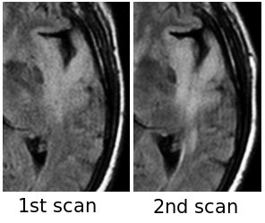
MR Flair images of a second grade astrocytoma:
(Left) image at the first examination (Right) image at the second examination.
In the anatomical MR images we observe the boundary
of the visible part of the tumor (the tumor delineation) rather than the tumor cell densities.
This discrepancy becomes crucial especially when one wants to extract model parameters from the images, in other words when solving the inverse problem. One solution to this problem might be to assume tumor cell density distributions based on the visible delineation. However, this adds extra assumptions about the image acquisition process. Our approach is to avoid this extra assumption and derive a reduced model. The definition of the reduced model is that it will formulate the evolution of the tumor delineation in time based on the same growth dynamics as the reaction-diffusion model. However, it will not use the information of tumor cell density distribution while doing so. Using the asymptotic properties of the reaction-diffusion equation we derive such a reduced model.
3.1. Asymptotic Properties of Reaction-Diffusion Equations
Convergence of Reaction-Diffusion Evolution
in the Infinite Cylinder: The PDE is initialized
with a compact support function and let evolve
in time on the left. It reaches its asymptotic
shape, the traveling wave. On the right we follow
the speed of the u=0.5 point, the blue dot on the
left. Observe that the speed of this point
approaches the asymptotic speed. |
|
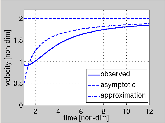
The speed of the traveling wave (shown in dark)
is time dependent and it converges to the asymptotic
speed (shown in dashed). The convergence is slow
therefore, we need to take it into account if we want
to approximate the speed of this wave.
The approximation we use takes this into account
(shown in dashed-dots). |
The reaction-diffusion equations have been analyzed thoroughly in the literature [Ebert and Saarlos, 2000],[Aronson and Wienberger, 1978]. Here we wish to recall some of the important characteristics of these equations, specifically for the Fisher-Kolmogorov equation in the infinite cylinder with constant coefficients D and ρ.

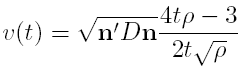
This equation models the change of tumor cell density distributions u. When it is initialized with a compact support initial condition u(t=0) and let evolve, the u distribution approaches to a traveling wave solution. This phenomenon is shown in the video at the right. The existence of the traveling wave solution also tells us that after long time the whole tumor profile will move at a constant speed. This asymptotic speed is given as a function of the coefficients of the PDE.
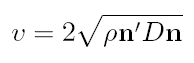
where
n is the direction of motion in the infinite cylinder. This asymptotic speed is also shown in the figure on the right. Now, we notice that when we follow a point on the tumor profile and look at its speed as a function of time (both shown in the video and also in the image) we observe the slow convergence to the asymptotic speed. Moreover, we notice that this function should depend on the u value of the point we follow. In [Ebert and Saarlos, 2000] this aspect is investigated and in that work it is stated that the convergence rate is in the order of O(1/t). Moreover the speed functions dependence on the value of u is on the order of 1/t
2. Based on the ideas presented in that reference we write an approximation for the speed of the tumor front which includes the slow convergence rate.
This time dependent approximation is shown in the figure on the right. We notice that this function well approximates the speed of the point u=0.5 on the tumor front. Here we assume that the tumor delineation visible in the images corresponds to an iso-density contour of the tumor cell distribution and we use the speed function v(t) to describe the evolution of the tumor delineation and creating our reduced model.
3.2. Eikonal Approximation for Tumor Growth
delineation in time based on the reaction-diffusion
dynamics. The traveling time formulation
is used for the evolution.","vid1-tumgro25")?>
The asymptotic properties of the reaction-diffusion equations provide us the basic foundation for creating the reduced model. The speed function defined in the previous section is assumed to describe the speed of the tumor delineation whose growth is defined by the reaction-diffusion process. We notice that in the previous section the speed function was defined for the reaction-diffusion equation in the infinite cylinder with constant coefficients. In order to generalize this case to tumor growth (which is not in the infinite cylinder and may have curved evolutions and the coefficients are at least spatially varying) we can apply certain assumptions (see [Konukoglu et al., 2007a]) and obtain the
traveling time formulation. Now if we use the asymptotic speed v to create the traveling time formulation we would obtain
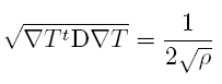
where T is the traveling time which denotes at a point x the time the tumor delineation will cover the point. This formulation is already very useful since it gives us a first reduced model. If we want to add the effect of time and convergence rate on the speed of the tumor delineation then we obtain
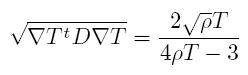
This form of the reduced model includes the rate of convergence and provides a better description for the motion of the tumor delineation. When we apply this formulation in the brain images we obtain simulations as seen in the video above. This reduced model formulates the evolution of the delineation of the tumor whose cell density evolution is modeled by the reaction-diffusion model. In the image below we compare for a synthetic tumor the evolution of the tumor delineation described by the reaction-diffusion model computed through thresholding tumor cell densities at u=0.4 (a normalized value consistent with the literature) and the evolution of the tumor delineation simulated by the reduced model which does not use the cell densities.
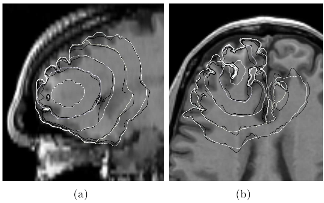
Comparison of the motion of the tumor delineation computed through simulations with reaction-diffusion model and thresholding the cell densities (in white) and the reduced model without using tumor cell densities (in black). We observe that the high similarity between the images. Each contour represents the position of the tumor delineation at a single time point from day 400 to 1200 as we move outwards.
3.3. References
- [Konukoglu et al., 2007a] Konukoglu, E., Sermesant, M., Clatz, O., Peyrat, JM, Delingette, H., Ayache, N., 2007. A recursive anisotropic fast marching approach to reaction diffusion equation: application to tumor growth modeling., IPMI 2007.
- [Ebert and Saarlos, 2000] U. Ebert, W.V. Saarloos,
2000. Front propagation into unstable states: universal algebraic convergence towards uniformly translating pulled fronts. Physica D: Nonlinear Phenomena, 146.
- [Aronson and Weinberger, 1978] ]D.G. Aronson and H.F. Weinberger, 1978. Multidimensional Nonlinear Diffusion Arising in Population Genetics. Advances in Mathematics, 1978, 30.