Computational Anatomy of the Brain
5. Spatiotemporal Atlas Estimation in Longitudinal Datasets
In the context of the Health-e-Child project, we aim at understanding the child brain maturation from an anatomical point of view. As emphasized by [Toga et al., 2006], "the dynamic course of brain maturation is one of the most fascinating aspects of the human condition. Although brain change and adaptation are part of a lifelong process, the earliest phases of maturation -during foetal development and childhood- are perhaps the most dramatic and important. Indeed, much of the potential and many of the vulnerabilities of the brain might, in part, depend on the first two decades of life." The newborn brain will grow up to a factor 3 or 4. During this period, the axons will be progressively myelinated and the brain will specialize according to both its genetic program and its environmental influences: the number of synaptic connections will dramatically increase whereas some connections will be removed to give a 'more efficient' set of connections.
Whereas the detailed maturation of the brain is obviously specific to every child we believe that there are some common features and that the normal maturation follows the same underlying standard process. Our goal is therefore to describe such a mean scenario and to analyze the deviations of a given brain maturation from this mean. With such statistical models we would be able to divide a given population into statistically consistent clusters, to classify new observations according to models learnt on large datasets, to analyze the correlations between brain growth and extrinsic features like gender or handedness, to detect abnormal evolutions as deviations from the normal models, to register atlas to patient's specific anatomy. Here, we face not only a high shape variability among different subjects (inter-subject variability) but also high variations of the same brain trough the time. The central issue is therefore to model the variability of geometric features evolutions (in a space of (3+1) dimensions) instead of the variability of the geometric feature at a given age (in a 3D space). Indeed, it seems not to be relevant to integrate individual measures of child brains independently at each age since the brain maturation stages appear at different ages, with different speed for every child. Instead of computing a mean shape of a given anatomical structure and analyzing the deviation of the anatomy around this mean, we would better compute a mean scenario and analyze the deviation both in space and time of the maturation process around this mean scenario.
In the previous section, we develop a complete statistical model that decomposes the variability of anatomical structure into a geometrical and a texture part. All the available information is taken into account: we can simulate new data according to our model. The experiments on the fiber bundles shows undoubtedly that both parts contains interesting anatomical features. They show the large range of possible variations that our model is able to retrieve. It comes from the fact that our model is not based on strong assumptions on the nature of the variability we are looking for.
However, this analysis could not be performed directly on temporal data that have not been registered in time. Our current work focus on extending this framework to account for temporal data. An observation is a couple shape plus time. Our extended framework will consist of a mean scenario (an evolving template) which account for all the temporal evolution and spatial deformation of this template which accounts for the inter-subject variability at every time points. Besides the usual spatial variability across subjects, the framework also enables to describe the variability in terms of speed growth via temporal registration. The whole section is based on the work presented in [Durrleman et al. MICCAI 2009].
5.1 Methodology for Statistics on Longitudinal Data
Many frameworks has been already proposed in medical imaging to analyze the anatomical variability of 3D structures like images, curves or surfaces. Less attention has been paid to the variability of longitudinal data (several subjects scanned several times). In [Qiu et al. 2008], the evolution between two shapes is modeled by a geodesic deformation, which cannot be used for more than two data per subjects. In [Gorczowski et al 2009], shape growth is measured via the evolution of extracted features like volumes, shape or pose parameters. In [Davis et al, 2007] and [Khan & Beg 2008], a temporal regression is proposed globally for a population, but this does not allow inter-subject comparisons. In cardiac motion analysis [Chandrashekara et al. 2003, Peyrat et al. 2008], spatiotemporal registration relies on 3D-registrations between images of the same moment of the cardiac cycle and between two consecutive time-points. These works rely on time-point correspondence and do not call the labels of the time-points into question. By contrast, in longitudinal studies, subjects are scanned at ages which do not necessarily correspond. Moreover, evolutions may be delayed or advanced within a population, a key feature that we precisely aim at detecting. In [Declerck et al. 1998, Perperidis et al. 2005], deformation of cardiac motion are proposed both in space and time but they require a fine temporal sampling of the motion, whereas only few acquisitions per subjects are available in most longitudinal studies. In this work, we propose to use a regression model to estimate a continuous evolution from data sparsely distributed in time and spatiotemporal deformations which register jointly both the 3D geometry and the scenario of evolution. Geometrical data are modeled as currents to avoid assuming point correspondence between structures. Large deformations are used which gives a rigorous framework for statistics on deformations and atlas construction. From longitudinal data, we estimate consistently the most likely scenario of evolution and its spatiotemporal variability within the population.
Here, we call longitudinal data a set of geometrical data (curves or surfaces, called here shapes), acquired from different subjects scanned at several time-points. We assume that the successive data of a given subject are temporal samples of a continuous evolution. We propose therefore a regression model which computes a continuous evolution which matches the data of the subject at the corresponding time points (Fig. 1). This continuous evolution allows us to compare two subjects at a given age, even if one subject has not been scanned at this age.We can also analyze how the shape varies near this age to detect possible developmental delays. We define then the spatiotemporal deformation of a continuous evolution, which consists of two deformations: (1) a morphological deformation (of the 3D space) which changes the geometry of every frame of the evolution independently of the time point and (2) a time change function (deformation of the time interval) which changes the dynamics of the evolution without changing the geometry of shapes. To avoid time-reversal, the time change function must be smooth and order preserving: it is a diffeomorphism of the time interval of interest. A 4D registration between two subjects looks for the most regular spatiotemporal deformation, such that the deformation of the continuous evolution inferred from the first subject maps the successive target data (Fig. 2). Eventually, we use this 4D registration framework to estimate a spatiotemporal atlas from a population, based on an 4D extension of the statistical model of [Durrleman et al. MEDIA 2009]. We look for a template and a continuous evolution of this template (called mean scenario of evolution), so that data of each subject are temporal samples of a spatiotemporal deformation of the mean scenario. A Maximum A Posteriori estimation enables to estimate consistently the template, the mean scenario and the spatiotemporal deformations of this mean scenario to each subject.
5.2 Regression Model for Shape Evolution
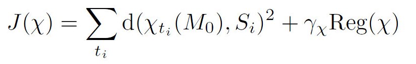
We want to fit a continuous shape evolution to a set of shapes (Si) of the same subject acquired at different time points (ti). Without loss of generality, we can assume that tmin = 0 and tmax = T. This evolving shape is equal to the baseline M0 at time t = 0, which may be the earliest shape of this subject or a template as in Sec. 5.4. The evolution has the form: Mt = χt(M0) where t varies continuously in the time interval [0, T]. For each t, χt is a diffeomorphism of the 3D space, such that χ0 = Id (which leads to χ0(M0) = M0). The regression (Mt) must match the observation Si at the time-points ti, while a rigidity constraint controls the regularity of the regression. This is achieved by minimizing:
5.3 Spatiotemporal Pairwise Registration
We assume now that we have successive shapes for the source subject Si=S(ti) and for the target Tj=T(tj). As in Sec 5.2, we perform a regression on the source shapes which leads to a continuous evolution S(t). Our goal is to find a diffeomorphism of the 3D space φ and a diffeomorphism of the time-interval ψ which deform the source evolution S(t) into S'(t) = φ(S(ψ(t))) such that S'(tj) match T(tj). Thanks to the regression function, no correspondence is needed between the time points ti and tj . Formally, we minimize:
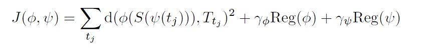
The spatial (resp. temporal) deformation φ (resp. ψ) is solution at parameter u = 1 of the flow equation ∂u φu(t)= vuψ(ψ(t)). The norm of the speed vector fields vφ and vψ integrated between 0 and 1 defines the regularity terms Reg(φ) and Reg(ψ) respectively. As in Sec 5.2, the geometrical (resp. temporal) deformation is parametrized by momenta α (resp. β) at the points of S(o) (resp. at the poinst of T(0)), which are used as variables for the gradient descent. Details are given in [Durrleman et al. MICCAI 2009]. We used here the fact that the shapes are embedded with a vector space (the space of currents) provided with an inner product. Note that we minimize J with respect to the geometrical and the temporal parameters jointly. We do not performed alternated minimization.
5.4 Spatiotemporal Atlas Construction
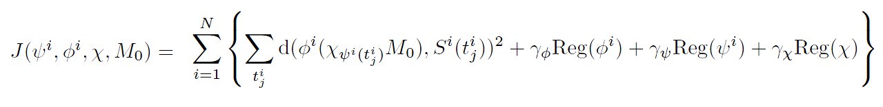
We assume now that we have a set of N subjects (Si), provided each with temporal observations (Si(tij). We are looking for a template M0 and a mean scenario of evolution of this template M(t) = χt(M0), such that the observations correspond to particular moments of a spatiotemporal deformation of the mean scenario. A Maximum A Posteriori estimation in the same setting as in [Durrleman et al. MEDIA 2009], leads to the minimization of
5.5 Numerical Experiments
Evolution of 2D Curves
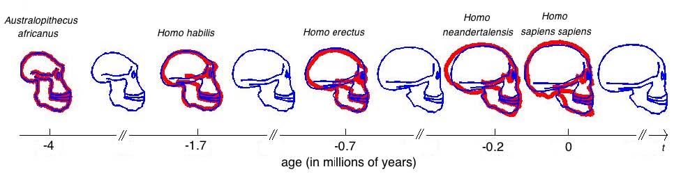
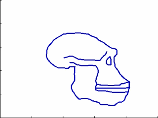
This experiments relates to Sec. 5.2 and 5.3. We have five 2D-profiles of hominids skulls which consist of six lines each (source: www.bordalierinstitute.com). Our regression framework infers a continuous evolution from the Australopithecus to the Homo sapiens sapiens which matches the intermediate stages of evolution in Fig. 1.
|
|
Then, we register the evolution {Homo habilis-Homo erectus-Homo neandertalensis} to the evolution {Homo erectus-Homo sapiens sapiens} in Fig 2.
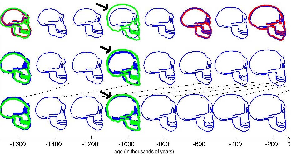
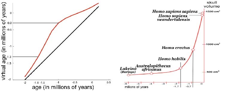
The geometrical deformation shows that during the later evolution the jaw was less prominent and the skull larger and rounder than during the earlier evolution. The time change function shows that the later evolution occurs at a speed 1.66 times faster than the earlier evolution. This value is compatible with the growth speed of the skull during these periods (See Fig. 3): between Homo erectus and sapiens the skull volume growths at (1500 − 900)/0.7 = 860cm3/106years, whereas between Homo habilis and neandertalensis, it growths at (1500 − 600)/1.7 = 530cm3/106years, namely 1.62 times faster.
Evolution of 3D surfaces
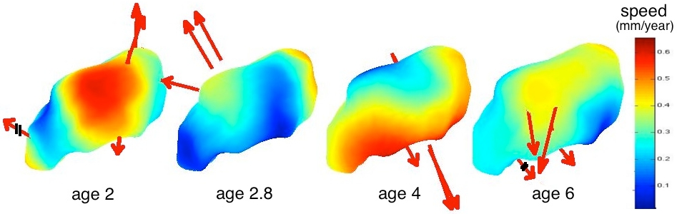
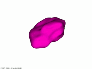
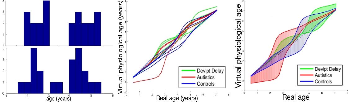
This experiment illustrates the complete spatiotemporal atlas construction detailed in Sec. 5.4 with surfaces extracted from brain images. We use here meshes of amygdala of the right hemisphere from 4 autistics, 4 developmental delay and 4 control children scanned twice [Hazlett et al. 2005]. Age distribution is shown in Fig 5-a. From these data registered rigidly, we infer a template, a mean scenario of evolution of this template and the spatiotemporal evolution of this mean scenario to each subject. In the setting of [Miller et al. 2002, Durrleman et al. MEDIA 2008], the diffeomorphisms are controlled by the standard deviation of Gaussian kernel set to 15 mm for χ, φand 1 year for ψ. The typical scale on currents is set to 3 mm. The trade-off parameters were set to γχ= 10-3 and γφ=10-6. An amygdala is typically 10 mm large. The discrete time step is set to 0.2 years.
|
|
By inspection of the companion movie of the mean scenario, one distinguishes 4 phases during growth (See also Fig. 4). Preliminary tests do not show correlations between the morphological deformations and the pathology. From the time change functions shown in Fig. 5, we cannot conclude that a subject with pathology is systematically delayed or advanced compared to controls, even at a given age. However, the curves show that the growth speed seems to follow the same pattern, mainly an acceleration between age 2.5 and 3.5 for the autistics and between age 4 and age 5 for controls. The developmental delay also have such pattern but it occurs at a very variable age. These results suggest that the discriminative information between classes might not be inferred from the anatomical variability at a given age, but rather from variations of the growth process. These results, however, must be strengthen using larger database. The more time-points per subjects, the more constrained the mean scenario estimation. The more subjects, the more robust the statistics.
5.6 Discussion and Conclusion
In this work, we proposed a generic framework to analyze variability of longitudinal data. A regression model fits a continuous evolution to successive data of one subject. 4D registrations decompose the difference between two sets of longitudinal data into a geometrical deformation and a change of the dynamics of evolution. The more acquisitions per subjects, the more constrained this decomposition. However, no constraint is imposed in terms of number and correspondence of measurement points across subjects. These pairwise registrations are used for group-wise statistics: ones estimates consistently a template, the mean evolution of this template and the spatiotemporal variability of this evolution in the population. Then, statistical measures can be derived, like the first mode of temporal deformation in Fig. 5. These first results suggest that pathologies might be characterized more by a particular scenario of evolution than by the anatomy at a given age. Our methodology can be used therefore to drive the search of new anatomical knowledge and to give characterization of pathologies in terms of organ growth scenario. This may be applied to the study of degenerative diseases or cardiac motion disorders.
5.7 References
- [Chandrashekara et al. 2003] Chandrashekara, R., Rao, A., Sanchez-Ortiz, G., Mohiaddin, R.H., Rueckert, D.: Construction of a statistical model for cardiac motion analysis using nonrigid image registration. In: Proc. of IPMI. Volume 2732 of LNCS., Springer (2003) 599-610
- [Davis et al. 2007] Davis, B., Fletcher, P., Bullitt, E., Joshi, S.: Population shape regression from random design data. In: Proc. of ICCV'07. 1-7
- [Declerck et al. 1998] Declerck, J., Feldman, J., Ayache, N.: Definition of a 4D continuous planispheric transformation for the tracking and the analysis of LV motion. Medical Image Analysis 4(1) (1998) 1-17
- [Durrleman et al. MEDIA 2008] Durrleman, S., Pennec, X., Trouvé, A., Thompson, P., Ayache, N.: Inferring brain variability from diffeomorphic deformations of currents: an integrative approach. Medical Image Analysis 12(5) (October 2008) 626-637
- [Durrleman et al. MICCAI 2008] Durrleman, S., Pennec, X., Trouvé, A., Ayache, N.: Sparse approximation of currents for statistics on curves and surfaces. In: Proc. of MICCAI'08. 390-398.
- [Durrleman et al. MEDIA 2009] Durrleman, S., Pennec, X., Trouvé, A., Ayache, N.: Statistical models of sets of curves and surfaces based on currents. Medical Image Analysis (2009).
- [Durrleman et al, MICCAI 2009] Durrleman, S., Pennec, X., Trouvé, A., Gerig, G., Ayache, N.: Spatiotemporal atlas estimation for developmental delay detection in longitudinal datasets. In Guang-Zhong Yang, David Hawkes, Daniel Rueckert, Alison Noble, and Chris Taylor, editors, Medical Image Computing and Computer-Assisted Intervention (MICCAI'09), Part I, volume 5761 of Lecture Notes in Computer Science, London, UK, pages 297-304, September 2009. Springer. Also as Research Report 6952, INRIA (06 2009)
- [Gorczowski et al. 2009] Gorczowski, K., Styner, M., Jeong, J.Y., Marron, J.S., Piven, J., Hazlett, H.C., Pizer, S.M., Gerig, G.: Statistical shape analysis of multi-object complexes. Transactions on Pattern Analysis and Machine Intelligence (2009).
- [Hazlett et al. 2005] Hazlett, H., Poe, M., Gerig, G., Smith, R., Provenzale, J., Ross, A., Gilmore, J., Piven, J.: Magnetic resonance imaging and head circumference study of brain size in autism. The Archives of General Psychiatry 62 (2005) 1366-1376
- [Khan & Beg 2008] Khan, A., Beg, M.: Representation of time-varying shapes in the large deformation diffeomorphic framework. In: Proc. of ISBI 2008. 1521-1524
- [Miller et al. 2002] Miller, M, I., Trouvé, A., Younes, L.: On the metrics and Euler-Lagrange equations of computational anatomy. Annual Review of Biomed. Eng. 4 (2002) 375-405
- [Perperidis et al. 2005] Perperidis, D., Mohiaddin, R.H., Rueckert, D.: Spatio-temporal free-form registration of cardiac MRI sequences. Medical Image Analysis 9(5) (2005) 441 - 456
- [Peyrat et al. 2008] Peyrat, J.M., Delingette, H., Sermesant, M., Pennec, X., Xu, C., Ayache, N.: Registration of 4D Time-Series of Cardiac Images with Multichannel Diffeomorphic Demons. In: Proc. MICCAI. Volume 5242 of LNCS., Springer (2008) 972-979
- [Qiu et al. 2008] Qiu, A., Younes, L., Miller, M., Csernansky, J.: Parallel transport in diffeomorphisms distinguishes the time-dependent pattern of hippocampal surface deformation due to healthy aging and the dementia of the alzheimer's type. NeuroImage 40 (2008) 68-76
- [Toga et al., 2006] Toga A.W, Thompson P.M., Sowell E.R., Mapping brain maturation, Trends in Neurosciences, 2006
- [Vaillant & Glaunès 2005] Vaillant, M., Glaunès, J.: Surface matching via currents. In: Proc. of IPMI'05. Volume 3565 of LNCS. (2005) 381-392