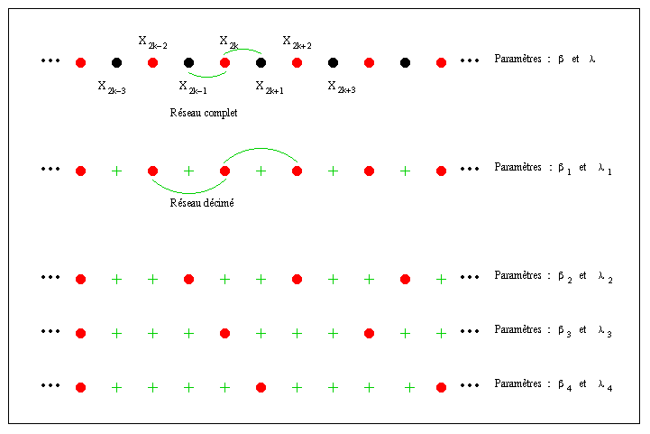


We shall keep the rational fractions that give the best compromise between a precise approximation of sqrt(2) and sqrt(5) and a small number of variables on which we have to integrate.


For pratical considerations we do not look for the equivalent parameters
in relation to the reference lattice. In fact we calculate the equivalent parameters
in relation to the lattice of step 1. We do this both for lattice of step sqrt(2) and for lattice
of step sqrt(5).
Thus we keep the conditional variances estimated in the directions
N/S and E/W, and we normalize the estimated conditional variances in all
the others directions. We use the reference lattice only for sake of easier
calculus.

So that we could point up the interest of the normalization we extract
a quasi-isotropic subimage from an urban area in the original image. Indeed
the distributions of the eight parameters should be the same for anfor
an isotropic image after the normalization.
So we draw the histograms of the conditional variances before normalization
and after normalization.
We calculate the Kolmogorov-Smirnov distance dKS between each distribution and the distribution of the conditional variance
estimated in the direction NE.
In fact the directions E and N are privileged directions. Both directions
correspond to the orientation of the streets and of the buildings. That
is why we only compare the
distributions corresponding to the 6 others directions. If the image
were exactly isotropic dKS between the distributions relating
to the directions NE and NW (lattices of same step sqrt(2)) should be zero before and after normalization.
In our test this value is 0.12 . This value is thus used as a reference
value to compare the others dKS . The dKS values decrease after
the normalization and are closer to the reference value 0.12. This points up the interest of such a normalization.
|
|
|
|
|
|
|
|
|
|
|
|
|
|
|
|
|
|
|
|
|
|
|
|
|
|
|
|
Last modified: Thu Sep 3 15:36:03 MET DST 1998